cs231n作业3笔记

简介

在作业 2 中手撸 CNN 后，cs231n 讲述了 RNN，LSTM，GRU 以及语言模型、图像标注、检测、定位、分割、识别等多方面的内容。

RNN captioning

常规 DNN 和 CNN 只能依次处理一个个的输入，输入之间是完全没有联系的，这对于图像分类的任务来说是没有问题的，但某些需要处理序列之间关系的任务而言就不适合了。例如：

图像标注问题(one to many)： image -> sequence of words
情感分类(many to one): sequence of words -> sentiment
机器翻译(many to many): seq of words -> seq of words
帧级别的视频分类(many to many)
……

为了更好地处理序列的信息，RNN(Recurrent Neural Network)诞生了。 RNN 需要预测一个和时间相关的量，其基本架构如下：

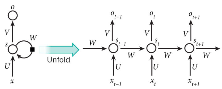
每个时间步都要根据前一个状态和当前输入计算一个新的状态。

\[ \boldsymbol{h}_t = f_W (\boldsymbol{h}_{t-1}, \boldsymbol{x}_t) \\ \downarrow \\ \boldsymbol{h}_t = tanh (\mathbf{W}_{hh}\boldsymbol{h}_{t-1} + \mathbf{W}_{xh} \boldsymbol{x}_t) \]

向上的箭头为每个时间步的输出，是一个 softmax 层

\[ \boldsymbol{y}_t = Softmax (\mathbf{W}_{hy} * \boldsymbol{h}_t) \]

根据上述公式，RNN 单元的 rnn_step_forward 如下：

prev_hWh = prev_h @ Wh                          # (1)
xWx = x @ Wx                                    # (2)
hsum = prev_hWh + xWx + b                       # (3)
next_h = np.tanh(hsum)                          # (4)

根据计算图反推，backward 也很简单：

dhsum = (1 - np.tanh(hsum)**2) * dnext_h      # (4)
dprev_hWh = dhsum                             # (3)
dxWx = dhsum                                  # (3)
db = np.sum(dhsum, axis=0)                    # (3)
dx = dxWx @ Wx.T                              # (2)
dWx = x.T @ dxWx                              # (2)
dWh = prev_h.T @ dprev_hWh                    # (1)
dprev_h = dprev_hWh @ Wh.T                    # (1)

接下来就是完整的 RNN 了，forward 过程需要对 RNN 单元循环 T 次（T为序列长度），在循环内部每次记得更新 $\boldsymbol{h}_t$ 即可。

backward 过程和以前的神经网络不太一样，RNN 从上游传过来的梯度不只一个，除了从右边传过来的梯度外，还有每个时间点（上面）传过来的梯度。首先需要逆序循环，然后每个循环内更新 RNN 单元需要的梯度值。此外，在 RNN 中，Wx, Wh, b 这三个参数是共享的，对每个时间步都是一样的，因此它们的梯度是一个累加的值。

dprev_ht = np.zeros((N, H))
for t in reversed(range(T)):
    dx[:, t, :], dprev_ht, dWxt, dWht, dbt = rnn_step_backward(
        dh[:, t, :] + dprev_ht, cache[t])
    dWx += dWxt
    dWh += dWht
    db += dbt
dh0 = dprev_ht

在用 RNN 对图像进行标注前，还需要进行词嵌入(word embeding)操作。神经网络不能将单词作为输入，所以需要将单词映射为单词索引的形式。

现在就可以来搭建 RNN 的架构了。首先需要把图像经 CNN 提取的特征（作业中采用的是在 ImageNet 数据集上预训练的 VGG16 模型的 fc7 层提取得到的特征）通过全连接层转换为初始的隐藏状态（$\boldsymbol{h}_0$），接着将 captions 做词嵌入输入 RNN 单元中，再利用一个仿射变换将 RNN 单元的输出转换为单词字典索引，接着采用 softmax 损失计算 loss。

h0, h0cache = affine_forward(features, W_proj, b_proj)
weout, wecache = word_embedding_forward(captions_in, W_embed)

if self.cell_type == 'rnn':
    rnnout, rnncache = rnn_forward(weout, h0, Wx, Wh, b)

x, xcache = temporal_affine_forward(rnnout, W_vocab, b_vocab)
loss, dx = temporal_softmax_loss(x, captions_out, mask)

上面描述的是 RNN 训练过程，测试时没有真值标注作为输入，需要一个起始单词（<START>）作为开始，然后按序列依次更新隐藏状态，并预测输出下一个标注单词。

prev_h, _ = affine_forward(features, W_proj, b_proj)
captions[:, 0] = self._start
x = self._start * np.ones((N, ), dtype=np.int32)
for t in range(1, max_length):
    embed, _ = word_embedding_forward(x, W_embed)

    if self.cell_type == 'rnn':
        next_h, _ = rnn_step_forward(embed, prev_h, Wx, Wh, b)

    prev_h = next_h
    out, _ = affine_forward(next_h, W_vocab, b_vocab)
    idx = np.argmax(out, axis=1)
    captions[:, t] = idx

LSTM captioning

RNN 应该能够记住许多时间步之前见过的信息，但实际中由于梯度消失（vanishing gradient problem）问题，随着层数的增加，网络将变得无法训练。LSTM(Long Short Term Memory)和 GRU 都是为了解决这个问题而提出的。

LSTM 单元结构如下：

forward 过程计算公式如下：

\[ \begin{align} \begin{pmatrix} i \\ f \\ o \\ g \end{pmatrix} & = \begin{pmatrix} \sigma \\ \sigma \\ \sigma \\ \tanh \end{pmatrix} \, \mathbf{W} \begin{pmatrix} h*{t-1} \\ x_t \end{pmatrix} \\ \\ c_t & = f \odot c*{t-1} + i \odot g \\ h_t & = o \odot \tanh(c_t) \end{align} \]

注意到每个 LSTM 单元有 3 个输入：$c, h, x$。实际计算时 4 个 gate 的线性部分可以通过一次计算完成，然后将不同 gate 对应的值分开即可。

H = prev_h.shape[1]
z = x @ Wx + prev_h @ Wh + b
igate = sigmoid(z[:, :H])
fgate = sigmoid(z[:, H:2 * H])
ogate = sigmoid(z[:, 2 * H:3 * H])
ggate = np.tanh(z[:, 3 * H:])

next_c = fgate * prev_c + igate * ggate
next_h = ogate * np.tanh(next_c)

backward 时，相比 RNN，反传过来的值有两个 dnext_h, dnext_c。求： dx, dWx, dWh, db, dprev_h 和 dprev_c 的梯度。弄清楚哪些变量之间有关联，然后利用链式法则即可：

dogate = dnext_h * np.tanh(next_c)
dnext_c += dnext_h * ogate * (1.0 - np.tanh(next_c)**2)
dfgate = dnext_c * prev_c
dprev_c = dnext_c * fgate
digate = dnext_c * ggate
dggate = dnext_c * igate

dz = np.zeros((N, 4 * H))
dz[:, :H] = digate * igate * (1.0 - igate)
dz[:, H:2 * H] = dfgate * fgate * (1. - fgate)
dz[:, 2 * H:3 * H] = dogate * ogate * (1.0 - ogate)
dz[:, 3 * H:4 * H] = dggate * (1.0 - ggate**2)

dx = dz @ Wx.T
dWx = x.T @ dz
dprev_h = dz @ Wh.T
dWh = prev_h.T @ dz
db = np.sum(dz, axis=0)

完整的 LSTM 大体和 RNN 相同，注意多了一个变量 c，不论是 forward 和 backward 都记得在循环里更新即可。

Network Visualization

之前训练模型都是利用 SGD 来更新模型参数使其达到损失函数定义下的要求。而在这一节中，我们利用已经训练好的预训练模型来定义相对于图像的损失函数，利用反向传播计算图像像素的梯度，保持模型不变，通过更新图像来最小化损失函数。

主要包括三个方面的内容：

显著性图（Saliency Maps）

显著性图告诉我们图像中每个像素影响图像类别分数的程度。通过计算正确类未规范化的分数相对于每个像素的梯度来得到。

scores = model(X) # correct class scores
scores = scores.gather(1, y.view(-1, 1)).squeeze() # backward
scores.backward(torch.ones(X.size(0)))

 # image gradient
saliency = X.grad

 # absolute the value and take the maximum value over the 3 channels
saliency = torch.abs(saliency)
saliency, _ = torch.max(saliency, dim=1)

Fooling images

Fooling images 则是在给定图像和类别时，通过梯度上升法不断地更新图像，最后使得模型认为该图像就是这个类别的图像为止。

while (True):
    scores = model(X*fooling)
    idx = torch.argmax(scores)

    if idx.item() == target_y:
        break

    scores[0, target_y].backward()

    dX = X_fooling.grad.data

    # update image using gradient ascent
    X_fooling.data += learning_rate * (dX / dX.norm())

    X_fooling.grad.zero_()

类别可视化（Class Visualization）

这里和 fooling images 差不多，都是预训练的模型通过梯度上升将输入的随机噪音图像变为指定类别的图像。

scores = model(img)
loss = scores[0, target_y] - l2_reg * img.norm()
loss.backward()
grad = img.grad.data
img.data += learning_rate * grad
img.grad.zero_()

Style Transfer

风格迁移的目的是将参考图像的风格应用于目标图像，同时保留目标图像的内容，从而生成一副新的图像。

风格迁移的思想与纹理生成的想法密切相关。实现风格迁移背后的关键思想与所有深度学习算法的思想一样：需要先定义一个损失函数定义要实现的目标，然后采用梯度下降法最小化这个损失函数。目标就是保存原始图像内容的同时实现风格化，若能在数学上给出 content 和 style 的定义，那么损失函数可以定义如下：

loss = distance(style(reference_image) - style(generated_image)) +
       distance(content(original_image) - content(generated_image))

这里的 distance 是一个范数，如 L2 范数。content 和 style 分别是计算输入图像内容和风格的函数。

content loss

内容损失描述的是网络从目标图像提取出的特征图与从生成图像提取的特征图之间的差别。通常选择的是靠近顶部的某一特征图来进行逐元素比较。代码如下：

def content_loss(content_weight, content_current, content_original):
    """
    Compute the content loss for style transfer.
    
    Inputs:
    - content_weight: Scalar giving the weighting for the content loss.
    - content_current: features of the current image; this is a PyTorch Tensor of shape
      (1, C_l, H_l, W_l).
    - content_target: features of the content image, Tensor with shape (1, C_l, H_l, W_l).
    
    Returns:
    - scalar content loss
    """
    loss = content_weight * torch.sum((content_current - content_original)**2)
    return loss

style loss

不同于内容损失，风格损失使用卷积网络的多个层来定义，以此来捕捉参考图像和生成图像上不同空间尺度上的信息。使用 Gram Matrix 来表示不同激活层之间的相关性：我们希望生成图像的激活统计量与风格图像的激活统计量相匹配。有很多种方法可以来表示这种相关，但 Gram Matrix 易于计算且效果很好。

对于 shape 为 $(C_l, M_l)$ 的特征图 $F^l$ ，其 Gram 矩阵 shape 为 $(C_l, C_l)$:

\[ G_{ij}^l = \sum_k {F_{ik}^l F_{jk}^l} \]

假定 $G^l$ 为当前图像的 Gram 矩阵，$A^l$ 为参考风格图像的特征图 Gram 矩阵，$w_l$ 为权重，那么 $l$ 层的风格损失可以简单的定义为两个 Gram 矩阵之间的欧氏距离：

\[ L_s^l = w_l \sum_{i,j} {(G_{ij}^l - A_{ij}^l)^2} \]

而风格损失是多个层的损失和：

\[ L_s = \sum_{l \in \mathcal{L}} {L_s^l} \]

首先实现 Gram 矩阵的计算：

def gram_matrix(features, normalize=True):
    """
    Compute the Gram matrix from features.
    
    Inputs:
    - features: PyTorch Tensor of shape (N, C, H, W) giving features for
      a batch of N images.
    - normalize: optional, whether to normalize the Gram matrix
        If True, divide the Gram matrix by the number of neurons (H * W * C)
    
    Returns:
    - gram: PyTorch Tensor of shape (N, C, C) giving the
      (optionally normalized) Gram matrices for the N input images.
    """
    N, C, H, W = features.size()
    features_reshaped = features.reshape(N, C, H * W)
    gram = torch.bmm(features_reshaped, features_reshaped.transpose(1, 2))
    if normalize:
        gram /= H * W * C
    return gram

接着，我们实现风格损失函数：

def style_loss(feats, style_layers, style_targets, style_weights):
    """
    Computes the style loss at a set of layers.
    
    Inputs:
    - feats: list of the features at every layer of the current image, as produced by
      the extract_features function.
    - style_layers: List of layer indices into feats giving the layers to include in the
      style loss.
    - style_targets: List of the same length as style_layers, where style_targets[i] is
      a PyTorch Tensor giving the Gram matrix of the source style image computed at
      layer style_layers[i].
    - style_weights: List of the same length as style_layers, where style_weights[i]
      is a scalar giving the weight for the style loss at layer style_layers[i].
      
    Returns:
    - style_loss: A PyTorch Tensor holding a scalar giving the style loss.
    """
    # Hint: you can do this with one for loop over the style layers, and should
    # not be very much code (~5 lines). You will need to use your gram_matrix function.
    loss = torch.FloatTensor([0]).type(dtype)
    for i, idx in enumerate(style_layers):
        gram = gram_matrix(feats[idx])
        loss += torch.sum(style_weights[i] * (gram - style_targets[i])**2)       
    return loss

Total-variation regularization

除了内容损失和风格损失之外，还需要添加一个全变分正则化损失，使生成图像的像素具有空间连续性和平滑，避免图像过度像素化。

全变分损失定义为水平和垂直方向相邻像素差的平方和，对于不同的通道之间也是相加。

def tv_loss(img, tv_weight):
    """
    Compute total variation loss.
    
    Inputs:
    - img: PyTorch Variable of shape (1, 3, H, W) holding an input image.
    - tv_weight: Scalar giving the weight w_t to use for the TV loss.
    
    Returns:
    - loss: PyTorch Variable holding a scalar giving the total variation loss
      for img weighted by tv_weight.
    """
    # Your implementation should be vectorized and not require any loops!
    hsum = torch.sum((img[:,:,:-1,:] - img[:,:,1:,:])**2)
    wsum = torch.sum((img[:,:,:,:-1] - img[:,:,:,1:])**2)
    return tv_weight * (hsum + wsum)

在风格迁移中，我们需要最小化的损失为内容损失、风格损失和全变差损失这三部分之和。接下来，只需要将这三部分组合起来，利用梯度下降法来得到最后的图像即可。具体可以参考 StyleTransfer-Pytorch.ipynb

GAN

在此之前，cs231n中所有的神经网络都是判别式模型，从给定的输入得到一个类别标记输出。其应用范围从图像分类到生成图像描述。在这一小节中，我们利用神经网络来构建生成模型。

2014年，Goodfellow et al.提出了训练生成模型的生成对抗网络（Generative Adversarial Networks，GAN）。在该方法中，需要构建两个不同的网络：第一个网络是传统的分类网络，称为判别器（discriminator），其功能是判断输入图像是真实的（输入训练集）还是假的（不属于训练集）。第二个网络称为生成器（generator），将随机噪声作为输入并产生一张图像。生成器的目标是骗过判别器，使其认为其生成的图像是真实的。

可以把判别器和生成器的博弈看作是一个最小最大的过程：

\[ \min_{G} \max_{D} \mathbb{E}_{x~p_{data}} \left[ \log D(x) \right] + \mathbb{E}_{z~p(z)} \left[ \log (1-D(G(z))) \right] \]

其中，$z~p(z)$ 为随机噪声样本，$G(z)$ 为生成器 $G$ 产生的图像，$D$ 为判别器的输出，表示输入为真实图像的概率。在Goodfellow et al.中，作者分析了这个最小最大过程和最小化训练数据分布与生成样本之间Jensen-Shannon散度的关联。

为了优化这个最小最大过程，可以选择对 $G$ 进行梯度下降优化，对 $D$ 进行梯度上升优化：

更新生成器 $G$ 使得判别器作出正确判断的概率最小
更新判别器 $D$ 使得判别器作出正确判断的概率最大

但是上述两个过程实际中难以work。因此，实际中更新生成器的准则是最大化判别器作出错误判断的概率。

该小节中，我们将交替执行如下更新：

最大化判别器作出错误判断的概率来更新生成器 $G$:

\[ \max_{G} \mathbb{E}_{z~p(z)} \left[ \log D(G(z)) \right] \]

最大化判别器在真实数据和生成数据上作出正确判断的概率来更新判别器 $D$

\[ \max_{D} \mathbb{E}_{x~p_{data}} \left[ \log D(x) \right] + \mathbb{E}_{z~p_{z}} \left[ \log (1-D(G(z))) \right] \]

实际上，自2014年GAN提出以来，有关GAN的论文层出不穷，相较于其他的生成模型，GAN能生成质量最高图像的同时，也需要高超的训练技巧。这个repo里包含了训练GAN的17个trick。提升GAN训练的稳定性和鲁棒性是一个开放的研究领域，每天都会用小的paper出来。最近的GAN教程，可以看这里。最近将目标函数变为Wasserstein距离的GAN模型（WGAN，WGAN-GP）获得了更稳定的结果。

需要注意的是，GAN不是训练生成模型的唯一方法！另一个流行的方法是变分自编码器（Variational Autoencoders）（由here 和 here共同发现）。VAE易于训练，但其生成的图像质量远不如GAN。

GAN的损失函数是用BCE（Binary Cross-Entropy）定义的，也即是对数回归的损失函数：

\[ bce(s,y) = -y * \log(s) - (1-y) * \log(1-s) \]

这里的$s$为经sigmoid函数作用后各个类别的分数，即 $s = \sigma(x)$，其值在0～1之间。那么直接计算bce loss 的时候就会有数值不稳定的问题：若s的值很小，那么 $\log(s)$ 便会接近 $-\infty$。因此，需做如下优化：

\[ \begin{align} & -y \log(\sigma(x)) - (1-y) \log(1 - \sigma(x)) \\ &= -y \log(\frac{1}{1+e^{-x}}) - (1-y) \log(e^{-x} - \frac{1}{1+e^{-x}}) \\ &= y \log(1 + e^{-x}) + (1 - y) (x + \log(1 + e^{-x})) \\ &= (1 - y) x + \log(1 + e^{-x}) \\ &= x - xy + \log(1 + e^{-x}) % 避免 x < 0时， exp(-x) 溢出 \\ &= -xy + \log(1 + e^x) \end{align} \]

为了确保稳定性，实现如下：

def bce_loss(input, target):
    """
    Numerically stable version of the binary cross-entropy loss function.

    As per https://github.com/pytorch/pytorch/issues/751
    See the TensorFlow docs for a derivation of this formula:
    https://www.tensorflow.org/api_docs/python/tf/nn/sigmoid_cross_entropy_with_logits

    Inputs:
    - input: PyTorch Tensor of shape (N, ) giving scores.
    - target: PyTorch Tensor of shape (N,) containing 0 and 1 giving targets.

    Returns:
    - A PyTorch Tensor containing the mean BCE loss over the minibatch of input data.
    """
    neg_abs = - input.abs()
    loss = input.clamp(min=0) - input * target + (1 + neg_abs.exp()).log()
    return loss.mean()

在此基础上，便可以分别实现判别器和生成器的损失函数了。这里就不贴代码了。后面的部分是介绍不同的GAN以及实现了。作业可以参考我的repo：GANs-Pytorch.ipynb

总结

作业3的内容更多的是将深度学习的多个应用展示一下，然后通过作业的形式来熟悉深度学习框架。涉及到的内容很丰富，想要深入理解的话，需要自己去查看相关文献才行。

至此，cs231n的作业笔记全部完成！🎉

文章目录

简介